液面高さの取得

2012年10月19日

はじめに

ある位置の液面高さの時系列データを得る方法について。

バージョン

OpenFOAM 2.1.1

液面高さの取得

interFoam の結果から ParaView により液面高さを取得することを考える。検討ケースとして、damBreak の初期条件で 0.1 の高さまで水を溜めたものを用意する。

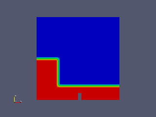
出力点を以下の 3 つとする。

0.291999995708466 0.00730000017210841
0.15 0.00730000017210841
0.45 0.00730000017210841

これを "points" ファイルとして以下で使用する。

ここでは重力方向は y 軸方向と想定する。

液面高さの取得方法として、以下の 2 つを検討する。

1. alpha1 を高さ方向に走査して 0.5 の位置を取り出す。
2. alpha1 を高さ方向に積分する。

1 は高さの座標が得られるのに対し、2 は底から液面までの距離が得られる。

方法 1

1. 結果を読み込む。"Cell Arrays" で "alpha1" のみを選択する。
2. 液面高さを取得する位置 (x, z) を定める。
3. Plot Over Line で (x, ymin, z) - (x, ymax, z) の上の数値データを CSV 形式で出力する。"Pass Partial Arrays" は off がよい。必要に応じて "Resolution" を設定する。
4. 数値データから alpha1 = 0.5 の位置を計算する。

出力点が大量にあると出力が大変なので、スクリプトを作る。

plot.py

import os

point_file = 'points'
output_file = 'plot.csv'
output_dir = './plot'


reader = OpenFOAMReader(FileName='case.foam')
#reader.CaseType = 'Decomposed Case' # for parallel
Show(reader)

reader.CellArrays = ['alpha1']

pol = PlotOverLine(reader)
Show(pol)

bounds = reader.GetDataInformation().GetBounds()
cx = (bounds[0] + bounds[1])/2.
cy = (bounds[2] + bounds[3])/2.
cz = (bounds[4] + bounds[5])/2.

ymin = bounds[2]
ymax = bounds[3]

pol.Source.Point1 = [cx, ymin, cz]
pol.Source.Point2 = [cx, ymax, cz]
pol.Source.Resolution = 100
pol.PassPartialArrays = 0

f = open('points', 'r')

i = 1
for line in f:
    line = line[:-1]
    item = line.split(' ')
    if len(item) == 2:
        x = float(item[0])
        z = float(item[1])

        pol.Source.Point1 = [x, ymin, z]
        pol.Source.Point2 = [x, ymax, z]

        Render()

        os.system('mkdir -p %s-%d' % (output_dir, i))

        w = CreateWriter('%s-%d/%s' % (output_dir, i, output_file))
        w.WriteAllTimeSteps = 1
        w.UpdatePipeline()

        i = i + 1

f.close()

exit()

ParaView 用 Python スクリプト。"points" ファイルから "x z" 形式の点座標を読み込み、点ごとにディレクトリ "plot-*" を作ってすべての時間ステップに対して CSV データを書き出す。並列ケースの場合はコメントをはずす。

getSurfaceHeight

#!/bin/sh
# get surface height

TIME_SCALE=0.05

# file name: *.<num>.csv
for FILE in *.csv ; do
    TIME_STEP=`echo $FILE | cut -d. -f2`
    TIME=`echo "$TIME_STEP * $TIME_SCALE" | bc`
    echo -n "$TIME "

    cat $FILE | awk -F',' '
BEGIN {
    hmax = -1e10;
    hmin = 1e10;
    amax = 0;
}
NR > 1 {
    if($1 >= 0.5 && $5 > hmax){
        hmax = $5;
        amax = $1;
    }
    if($1 < 0.5 && $5 < hmin){
        hmin = $5;
        amin = $1;
    }
}
END{
    if(amax == 0){
        print hmin;
    }else{
        print (hmax - hmin)/(amax - amin)*(0.5 - amin) + hmin;
    }
}'
done | sort -n

すべての時間ステップの CSV データから液面高さを計算し、"時間 高さ" のリスト "height" を出力する。TIME_SCALE に出力時間間隔を設定する。

runPlot

#!/bin/sh

paraview --script=plot.py

for DIR in plot-* ; do
    echo $DIR
    cd $DIR
    ../getSurfaceHeight > height
    cd ..
done

ParaView 用 Python スクリプト実行から、各点の "時間 高さ" リストを作るまでを行うスクリプト。

plotGraph

#!/usr/bin/gnuplot

set xlabel 'Time [s]'
set ylabel 'Height [m]'
set terminal png
set output 'plot.png'
plot 'plot-1/height' w l, 'plot-2/height' w l, 'plot-3/height' w l

gnuplot でグラフの絵を作るスクリプト。

方法 2

1. 結果を読み込む。"Cell Arrays" で "alpha1" のみを選択する。
2. 液面高さを取得する位置 (x, z) を定める。
3. Plot Over Line で (x, ymin, z) - (x, ymax, z) の線を設定する。"Pass Partial Arrays" は off がよい。
4. Integrate Variables で積分する。
5. Plot Selection Over Time で積分値の時系列データを作成し、CSV で出力する。データの選択は、Integrate Variables を Spread Sheet で表示させ、行を選択して行う。

出力点が大量にあると出力が大変なので、スクリプトを作る。

plot.py

import os

point_file = 'points'
output_file = 'plot'
output_dir = './plot'

reader = OpenFOAMReader(FileName='case.foam')
#reader.CaseType = 'Decomposed Case' # for parallel
Show(reader)

reader.CellArrays = ['alpha1']

pol = PlotOverLine(reader)
Show(pol)

bounds = reader.GetDataInformation().GetBounds()
cx = (bounds[0] + bounds[1])/2.
cy = (bounds[2] + bounds[3])/2.
cz = (bounds[4] + bounds[5])/2.

ymin = bounds[2]
ymax = bounds[3]

pol.Source.Point1 = [cx, ymin, cz]
pol.Source.Point2 = [cx, ymax, cz]
pol.PassPartialArrays = 0

iv = IntegrateVariables(pol)

v = paraview.simple._create_view('SpreadSheetView')

Show(iv)

psot = PlotSelectionOverTime(iv)

idss = IDSelectionSource()
idss.FieldType = 'POINT'
idss.IDs = [-1L, 0L]

psot.Selection = idss

Show(psot)

Render()

os.system('mkdir -p %s' % (output_dir))

f = open('points', 'r')

i = 1
for line in f:
    line = line[:-1]
    item = line.split(' ')
    if len(item) == 2:
        x = float(item[0])
        z = float(item[1])

        pol.Source.Point1 = [x, ymin, z]
        pol.Source.Point2 = [x, ymax, z]

        w = CreateWriter('%s/%s.%d..csv' % (output_dir, output_file, i))
        w.UpdatePipeline()

    i = i + 1

f.close()

exit()

ParaView 用 Python スクリプト。"points" ファイルから "x z" 形式の点座標を読み込み、ディレクトリ "plot" を作って点ごとに CSV データを書き出す。並列ケースの場合はコメントをはずす。

getSurfaceHeight

#!/bin/sh
# get surface height

for FILE in *.csv ; do
    NAME=`echo $FILE | cut -d. -f2`
    cat $FILE | awk -F',' 'NR > 1 { print $4, $1 }' > height.$NAME
doned

すべての CSV データから "時間 高さ" のリスト "height.*" を作る。

runPlot

#!/bin/sh

paraview --script=plot.py

cd plot
../getSurfaceHeight
cd ..

ParaView 用 Python スクリプト実行から、各点の "時間 高さ" リストを作るまでを行うスクリプト。

plotGraph

#!/usr/bin/gnuplot

set xlabel 'Time [s]'
set ylabel 'Height [m]'
set terminal png
set output 'plot.png'
plot 'plot/height.1' w l, 'plot/height.2' w l, 'plot/height.3' w l

gnuplot でグラフの絵を作るスクリプト。

結果

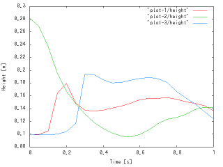
左が方法 1 の結果、右が方法 2 の結果。1 点目のグラフが異なるのは、1 点目がモデルの中央にあり、底が高くなっているからである。

おまけ

方法 1 の手順によるプログラムを作ってみた。

• getSurfaceHeight.tar.gz

ケースファイルで実行すると、"points" ファイルを読み込んで "plot.txt" ファイルを書き出す。

処理に時間がかかる場合、もしメッシュが途中で変わらないのであれば、以下の行をコメントにすると速くなる。

        // Check for new mesh
        mesh.readUpdate();