ミキシングエルボーの熱流動解析

2016年12月9日

はじめに

ミキシングエルボー内の熱流動解析の手順を示す。

使用バージョン

OpenFOAM 4.1

ファイル

• simpleFoam: mixing_elbow-simpleFoam-4.1.tar.gz
• buoyantPimpleFoam: mixing_elbow_heat-buoyantPimpleFoam-4.1.tar.gz

解析条件

モデルの寸法を下図に示す。

左下の入り口を in1、右下の入り口を in2 とする。右上を出口 out とする。

設定条件は以下とする。

• 流体は空気
• in1 : 0.2 m/s、20 ℃
• in2 : 1 m/s、40 ℃
• out : 大気圧
• 壁面 : non slip、断熱

simpleFoam による定常等温流動計算と buoyantPimpleFoam による非定常熱流動計算を行う。

計算の手順

計算の手順を下図に示す。

計算条件の設定の手順を下図に示す。

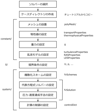
各項目の詳細については、以下を参照。

• 新しいケースの作成
• 物性値の設定
• 重力の設定
• 乱流モデルの設定
• 境界条件の設定
• 離散化スキームの設定
• 代数方程式ソルバーの設定
• 圧力-速度連成手法の設定
• 計算の制御の設定
• 初期値の設定
• ソルバーの実行
• 計算の確認と計算結果の処理

メッシュ

メッシュについては、すでに snappyHexMesh などで作成されているものとする (snappyHexMesh による作り方は こちら)。

snappyHexMesh の場合、blockMeshDict で境界に名前を付けていると、ケースディレクトリの constant/polyMesh/boundary に不必要な名前が残ることがあるため、それらを削除しておく。また、"mixing_elbow.stl" の中で境界名 "in1"、"in2" などとつけていると boundary では "mixing_elbow_in1"、"mixing_elbow_in2" などという名前になるため、短く "in1"、"in2" などに変更しておく。サンプルケースでは createPatch (設定は system/createPatchDict) でこれを行っている。

定常流動計算

定常 (等温) 流動計算を行うためには、simpleFoam を用いる (下図)。

設定は simpleFoam のチュートリアルケース motorBike をベースにする。

$ cp -r $FOAM_TUTORIALS/incompressible/simpleFoam/motorBike mixing_elbow

メッシュの設定を行ったあと、各種設定を行う。

物性値の設定

constant/transportProperties

transportModel  Newtonian;

nu              nu [0 2 -1 0 0 0 0] 1.5e-05;

物性は空気として動粘性係数 nu に 1.5e-05 を設定する。

重力の設定

simpleFoam では、重力の設定は必要ない。

乱流モデルの設定

constant/turbulenceProperties

simulationType RAS;

RAS
{
    RASModel            kEpsilon;

    turbulence          on;

    printCoeffs         on;
}

ここでは標準 k-εモデルを設定する。

バージョン 2.x の場合は RASProperties で設定する。

constant/RASProperties

RASModel            kEpsilon;

turbulence          on;

printCoeffs         on;

境界条件の設定

0 ディレクトリ内のフィールドファイルで境界条件を設定する。以下では 0 ディレクトリとしているが、ソルバーがフィールドファイルを勝手に書き換えることがあるので、0.org としてオリジナルを用意しておいて、ソルバー実行時に 0.org を 0 ディレクトリとしてコピーしたほうがよい。

0/U

FoamFile
{
    version     2.0;
    format      ascii;
    class       volVectorField;
    object      U;
}

dimensions      [0 1 -1 0 0 0 0];

internalField   uniform (0 0 0);

boundaryField
{
    #includeEtc "caseDicts/setConstraintTypes"

    ".*"
    {
        type            noSlip;
    }

    in1
    {
        type            fixedValue;
        value           uniform (0.2 0 0);
    }

    in2
    {
        type            fixedValue;
        value           uniform (0 0 1);
    }

    out
    {
        type            zeroGradient;
    }
}

流速の設定。in1、in2 に流入速度をベクトルで指定している。out は勾配 0 とする。"#includeEtc" の行は次の書き方と同じである。

    #include "${WM_PROJECT_DIR}/etc/caseDicts/setConstraintTypes"

境界条件タイプ noSlip は次の書き方と同じである。

    ".*"
    {
        type            fixedValue;
        value           uniform (0 0 0);
    }

0/p

FoamFile
{
    version     2.0;
    format      ascii;
    class       volScalarField;
    object      p;
}

dimensions      [0 2 -2 0 0 0 0];

internalField   uniform 0;

boundaryField
{
    #includeEtc "caseDicts/setConstraintTypes"

    ".*"
    {
        type            zeroGradient;
    }

    out
    {
        type            fixedValue;
        value           uniform 0;
    }
}

out に圧力 0 を設定する。

0/k

FoamFile
{
    version     2.0;
    format      ascii;
    class       volScalarField;
    object      k;
}

dimensions      [0 2 -2 0 0 0 0];

internalField   uniform 0.00015; // U = 0.2;

boundaryField
{
    #includeEtc "caseDicts/setConstraintTypes"

    ".*"
    {
        type            kqRWallFunction;
        value           $internalField;
    }

    in1
    {
        type            turbulentIntensityKineticEnergyInlet;
        intensity       0.05;
        value           $internalField;
    }

    in2
    {
        type            turbulentIntensityKineticEnergyInlet;
        intensity       0.05;
        value           $internalField;
    }

    out
    {
        type            zeroGradient;
    }
}

in1、in2 には乱れ強さ 5% を設定している。internalField には乱れ強さを 5%、流速を 0.2 m/s として見積もった k の値を設定している。

0/epsilon

FoamFile
{
    version     2.0;
    format      ascii;
    class       volScalarField;
    object      epsilon;
}

dimensions      [0 2 -3 0 0 0 0];

internalField   uniform 0.000431;

boundaryField
{
    #includeEtc "caseDicts/setConstraintTypes"

    ".*"
    {
        type            epsilonWallFunction;
        value           $internalField;
    }

    in1
    {
        type            turbulentMixingLengthDissipationRateInlet;
        mixingLength    0.0007;
        value           $internalField;
    }

    in2
    {
        type            turbulentMixingLengthDissipationRateInlet;
        mixingLength    0.00035;
        value           $internalField;
    }

    out
    {
        type            zeroGradient;
    }
}

in1、in2 にそれぞれの径を代表長さ L とした混合長 (0.07*L) を設定している。internalField には k と混合長から見積もったεの値を設定している。

0/nut

FoamFile
{
    version     2.0;
    format      ascii;
    class       volScalarField;
    location    "0";
    object      nut;
}

dimensions      [0 2 -1 0 0 0 0];

internalField   uniform 0;

boundaryField
{
    #includeEtc "caseDicts/setConstraintTypes"

    ".*"
    {
        type            nutkWallFunction;
        value           $internalField;
    }

    in1
    {
        type            calculated;
        value           uniform 0;
    }

    in2
    {
        type            calculated;
        value           uniform 0;
    }

    out
    {
        type            calculated;
        value           uniform 0;
    }
}

壁に壁関数を設定し、in1, in2, out は calculated としている。

離散化スキームの設定

system/fvSchemes

ddtSchemes
{
    default         steadyState;
}

...

divSchemes
{
    default         none;
    div(phi,U)      bounded Gauss upwind;
    div(phi,k)      bounded Gauss upwind;
    div(phi,epsilon)  bounded Gauss upwind;
    div((nuEff*dev2(T(grad(U))))) Gauss linear;
    div(div(phi,U)) Gauss linear;  // for potentialFoam
}

定常なので ddtSchemes に "steadyState" を設定する。divSchemes に必要な項目を追加し、対流項 ("phi" を含むもの) に upwind を設定する。motorBike では omega が使われているので、上記では epsilon に書き換えている。また、初期値を作成する potentialFoam のために 1 行追加している。

バージョン 2.x では粘性項の書き方が少し違っている。

system/fvSchemes

divSchemes
{
    default         none;
    div(phi,U)      bounded Gauss upwind;
    div(phi,k)      bounded Gauss upwind;
    div(phi,epsilon)  bounded Gauss upwind;
    div((nuEff*dev(T(grad(U))))) Gauss linear;
}

代数方程式ソルバーの設定

代数方程式ソルバー (system/fvSolution) については、結果にあまり影響しないため、適当なものを設定すればよい。ただし、motorBike では omega が使われているので、epsilon に書き換える必要がある。

圧力-速度連成手法の設定

system/fvSolution

SIMPLE
{
    nNonOrthogonalCorrectors 0;

    residualControl
    {
        p               1e-3;
        U               1e-3;
        "(k|epsilon)"   1e-3;
    }
}

relaxationFactors
{
    fields
    {
        p               0.3;
    }
    equations
    {
        U               0.7;
        "(k|epsilon)"   0.7;
    }
}

収束判定と緩和係数を適当に設定する。nNonOrthogonalCorrectors はメッシュ品質に応じて設定する。

計算の制御

system/controlDict

application     simpleFoam;

startFrom       latestTime;

startTime       0;

stopAt          endTime;

endTime         1000;

deltaT          1;

writeControl    timeStep;

writeInterval   100;

purgeWrite      2;

writeFormat     ascii;

writePrecision  6;

writeCompression uncompressed;

timeFormat      general;

timePrecision   6;

runTimeModifiable true;

定常計算なので、deltaT を 1 にする。endTime は 1000 程度にしておく。途中結果はすべて必要なわけではないので、purgeWrite に 2 を設定する。

初期値の設定

potentialFoam を実行して初期値を作る。

system/fvSolution

potentialFlow
{
    nNonOrthogonalCorrectors 10;
}

実行。

$ potentialFoam -writep

ソルバーの実行

simpleFoam を実行する。

$ simpleFoam > log &

あるいは、つぎのようにする。

$ foamJob simpleFoam

残差の確認

残差を確認するために foamLog を実行する。

$ foamLog log

各変数の残差が "logs" というディレクトリに格納される。これを gnuplot で描画すると、下図が得られる。

結果の確認

ParaView を起動して結果を確認する。

$ paraFoam

断面の流速は下図のようになる。

非定常熱流動計算

非定常熱流動計算を行うためには、buoyantPimpleFoam を用いる (下図)。

設定は buoyantPimpleFoam のチュートリアルケース hotRoom をベースにする。

$ cp -r $FOAM_TUTORIALS/heatTransfer/buoyantPimpleFoam/hotRoom mixing_elbow_heat

メッシュの設定を行ったあと、各種設定を行う。

物性値の設定

constant/thermophysicalProperties

thermoType
{
    type            heRhoThermo;
    mixture         pureMixture;
    specie          specie;
    equationOfState perfectGas;
    transport       const;
    thermo          hConst;
    energy          sensibleEnthalpy;
}

pRef            100000;

mixture
{
    specie
    {
        nMoles          1;
        molWeight       28.9;
    }
    thermodynamics
    {
        Cp              1000;
        Hf              0;
    }
    transport
    {
        mu              1.8e-05;
        Pr              0.7;
    }
}

物性は空気として、hotRoom に設定してあるものをそのまま使う。

重力の設定

constant/g

dimensions      [0 1 -2 0 0 0 0];

value           (0 0 -9.81);

図の下方向 (-Z 方向) に重力加速度を設定する。理想気体の状態方程式を用いるため、温度変化により密度が変化し、多少浮力が効く。

乱流モデルの設定

constant/turbulenceProperties

simulationType  RAS;

RAS
{
    RASModel        kEpsilon;

    turbulence      on; 

    printCoeffs     on; 
}

非定常 RANS モデルを用いる。ここでは標準 k-εモデルを設定する。

バージョン 2.x だと、設定ファイルが 2 つに分かれている。

constant/turbulenceProperties

simulationType  RASModel;

constant/RASProperties

RASModel            kEpsilon;

turbulence          on;

printCoeffs         on;

境界条件の設定

0/U

FoamFile
{
    version     2.0;
    format      ascii;
    class       volVectorField;
    object      U;
}

dimensions      [0 1 -1 0 0 0 0];

internalField   uniform (0 0 0);

boundaryField
{
    #includeEtc "caseDicts/setConstraintTypes"

    ".*"
    {
        type            noSlip;
    }

    in1
    {
        type            fixedValue;
        value           uniform (0.2 0 0);
    }

    in2
    {
        type            fixedValue;
        value           uniform (0 0 1);
    }

    out
    {
        type            zeroGradient;
    }
}

simpleFoam の設定と同じである。

0/p_rgh

FoamFile
{
    version     2.0;
    format      ascii;
    class       volScalarField;
    object      p;
}

dimensions      [1 -1 -2 0 0 0 0];

internalField   uniform 101325;

boundaryField
{
    #includeEtc "caseDicts/setConstraintTypes"

    ".*"
    {
        type            fixedFluxPressure;
        value           $internalField;
    }

    out
    {
        type            fixedValue;
        value           uniform 101325;
    }
}

out に大気圧を設定する。

0/p

FoamFile
{
    version     2.0;
    format      ascii;
    class       volScalarField;
    object      p;
}

dimensions      [1 -1 -2 0 0 0 0];

internalField   uniform 101325;

boundaryField
{
    #includeEtc "caseDicts/setConstraintTypes"

    ".*"
    {
        type            calculated;
        value           $internalField;
    }
}

p には特に境界条件の設定は必要ない。

0/T

FoamFile
{
    version     2.0;
    format      ascii;
    class       volScalarField;
    object      T;
}

dimensions      [0 0 0 1 0 0 0];

internalField   uniform 293;

boundaryField
{
    #includeEtc "caseDicts/setConstraintTypes"

    ".*"
    {
        type            zeroGradient;
    }

    in1
    {
        type            fixedValue;
        value           uniform 293;
    }

    in2
    {
        type            fixedValue;
        value           uniform 313;
    }
}

in1、in2 に流入温度を設定している。初期温度は in1 の温度としている。

0/k

FoamFile
{
    version     2.0;
    format      ascii;
    class       volScalarField;
    object      k;
}

dimensions      [0 2 -2 0 0 0 0];

internalField   uniform 0.00015; // U = 0.2;

boundaryField
{
    #includeEtc "caseDicts/setConstraintTypes"

    ".*"
    {
        type            kqRWallFunction;
        value           $internalField;
    }

    in1
    {
        type            turbulentIntensityKineticEnergyInlet;
        intensity       0.05;
        value           $internalField;
    }

    in2
    {
        type            turbulentIntensityKineticEnergyInlet;
        intensity       0.05;
        value           $internalField;
    }

    out
    {
        type            zeroGradient;
    }
}

simpleFoam の設定と同じ。バージョン 2.x の場合、"kqRWallFunction" の頭に "compressible::" が必要。

0/epsilon

FoamFile
{
    version     2.0;
    format      ascii;
    class       volScalarField;
    object      epsilon;
}

dimensions      [0 2 -3 0 0 0 0];

internalField   uniform 0.000431;

boundaryField
{
    #includeEtc "caseDicts/setConstraintTypes"

    ".*"
    {
        type            epsilonWallFunction;
        value           $internalField;
    }

    in1
    {
        type            turbulentMixingLengthDissipationRateInlet;
        mixingLength    0.0007;
        value           $internalField;
    }

    in2
    {
        type            turbulentMixingLengthDissipationRateInlet;
        mixingLength    0.00035;
        value           $internalField;
    }

    out
    {
        type            zeroGradient;
    }
}

simpleFoam の設定と同じ。バージョン 2.x の場合、type の設定の頭にそれぞれ "compressible::" が必要。

0/nut

FoamFile
{
    version     2.0;
    format      ascii;
    class       volScalarField;
    location    "0";
    object      nut;
}

dimensions      [0 2 -1 0 0 0 0];

internalField   uniform 0;

boundaryField
{
    #includeEtc "caseDicts/setConstraintTypes"

    ".*"
    {
        type            nutkWallFunction;
        value           $internalField;
    }

    in1
    {
        type            calculated;
        value           uniform 0;
    }

    in2
    {
        type            calculated;
        value           uniform 0;
    }

    out
    {
        type            calculated;
        value           uniform 0;
    }
}

simpleFoam の設定と同じ。

0/alphat

FoamFile
{
    version     2.0;
    format      ascii;
    class       volScalarField;
    location    "0";
    object      alphat;
}

dimensions      [1 -1 -1 0 0 0 0];

internalField   uniform 0;

boundaryField
{
    #includeEtc "caseDicts/setConstraintTypes"

    ".*"
    {
        type            compressible::alphatJayatillekeWallFunction;
        value           $internalField;
        Prt             0.85;
    }

    in1
    {
        type            calculated;
        value           uniform 0;
    }

    in2
    {
        type            calculated;
        value           uniform 0;
    }

    out
    {
        type            calculated;
        value           uniform 0;
    }
}

離散化スキームの設定

system/fvSchemes

ddtSchemes
{
    default         Euler;
}

...

divSchemes
{
    default         none;
    div(phi,U)      Gauss upwind;
    div(phi,h)      Gauss upwind;
    div(phi,e)      Gauss upwind;
    div(phi,k)      Gauss upwind;
    div(phi,epsilon) Gauss upwind;
    div(phi,R)      Gauss upwind;
    div(phi,K)      Gauss linear;
    div(phi,Ekp)    Gauss linear;
    div(R)          Gauss linear;
    div(((rho*nuEff)*dev2(T(grad(U))))) Gauss linear;
}

非定常なので ddtSchemes に "Euler" を設定する。divSchemes に必要な項目を追加し、対流項 ("phi" を含むもの) に upwind を設定する。

バージョン 2.x では粘性項の書き方が少し違っている。

system/fvSchemes

divSchemes
{
    default         none;
    div(phi,U)      Gauss upwind;
    div(phi,h)      Gauss upwind;
    div(phi,K)      Gauss upwind;
    div(phi,k)      Gauss upwind;
    div(phi,epsilon) Gauss upwind;
    div((muEff*dev2(T(grad(U))))) Gauss linear;
}

代数方程式ソルバーの設定

simpleFoam の場合と同様、代数方程式ソルバー (system/fvSolution) については、結果にあまり影響しないため、適当なものを設定すればよい。

圧力-速度連成手法の設定

system/fvSolution

PIMPLE
{
    momentumPredictor yes;
    turbOnFinalIterOnly yes;
    nOuterCorrectors 1;
    nCorrectors     2;
    nNonOrthogonalCorrectors 0;

    residualControl
    {
        p
        {
            relTol          0.05;
            tolerance       1e-3;
        }
        U
        {
            relTol          0.05;
            tolerance       1e-3;
        }
        h
        {
            relTol          0.05;
            tolerance       1e-3;
        }
        "(k|epsilon)"
        {
            relTol          0.05;
            tolerance       1e-3;
        }
    }
}

relaxationFactors
{
    fields
    {
        p_rgh           0.3;
    }
    equations
    {
        U               0.7;
        h               0.7
        "(k|epsilon)"   0.7;
        ".*Final"       1;
    }
}

収束判定と緩和係数を適当に設定する。nNonOrthogonalCorrectors はメッシュ品質に応じて設定する。ここでは nOuterCorrectors を 1 に設定しているため PISO モードとなり、緩和係数は ".*Final" のものが使われる (つまり緩和は効かない)。

計算の制御

system/controlDict

application     buoyantPimpleFoam;

startFrom       latestTime;

startTime       0;

stopAt          endTime;

endTime         1;

deltaT          1e-3;

writeControl    adjustableRunTime;

writeInterval   0.1;

purgeWrite      0;

writeFormat     ascii;

writePrecision  6;

writeCompression off;

timeFormat      general;

timePrecision   6;

runTimeModifiable true;

adjustTimeStep  on;

maxCo           0.9;

1 秒間計算するために endTime に 1 を設定する。時間刻みの自動調整を使うために adjustTimeStep を "on" に設定し、deltaT に小さめの初期時間刻み幅 1e-3 を設定する。

初期値の設定

静止場からの非定常的な流れを見るため、初期値はフィールドファイルで設定したものをそのまま用いる。

もし定常状態から計算したい場合は、定常計算の結果をマッピングすることもできる。

$ mapFields ../mixing_elbow -sourceTime latestTime -consistent

ただし、圧力 p の扱い方が異なるため、p の値をそのまま用いることはできないので、本来の初期設定に戻す必要がある。

$ cp 0.org/p 0/p

ソルバーの実行

buoyantPimpleFoam を実行する。

$ buoyantPimpleFoam > log &

あるいは、つぎのようにする。

$ foamJob buoyantPimpleFoam

並列実行したい場合は、system/decomposeParDict を用意する。

system/decomposeParDict

FoamFile
{
    version     2.0;
    format      ascii;
    class       dictionary;
    object      decomposeParDict;
}

numberOfSubdomains 2;

method          scotch;

numberOfSubdomains に並列数を設定して、decomposePar で領域分割する。

$ decomposePar

MPI により実行。

$ mpirun -np 2 buoyantPimpleFoam -parllel

あるいは、つぎのようにする。

$ foamJob -p buoyantPimpleFoam

計算が終わったら、領域を結合する。

$ reconstructPar

結果の確認

ParaView を起動して結果を確認する。

$ paraFoam

断面の流速と温度 (摂氏) はそれぞれ下図のようになる。

非定常計算なので、時系列データから動画を作ることができる。ParaView のメニュー [Sources]-[Annotate Time] で時刻を表示させる。メニュー [File]-[Save Animation] で絵のサイズを設定し、ディレクトリを指定するとそこに画像が保存される。JPEG として保存すれば、つぎのように実行すると GIF アニメーションを作成できる。

$ convert *.jpg anime.gif

ただし、このコマンドを使うには ImageMagick がインストールされている必要がある。作成されたアニメーションは下図のようになる。

また、つぎのように実行すれば MPEG ファイルを作ることもできる。

$ convert *.jpg anime.mpeg

ただし、これもまた FFmpeg などに依存しているため、必要なパッケージがインストールされている必要がある。

古い

• OpenFOAM 2.2.2